Motion tracking with the Lucas-Kanade algorithm (with code)

To quickly get what we are talking about, take a look at this video:

Now, let’s clarify some jargon issues. We are talking about optical flow algorithms. And, when one talks about optical flow algorithms, they are almost always referring to dense optical flow. In that case, the optical flow is computed all across an image (actually, a pair of images) and yields a velocity field. The figure below illustrates that well: the bottom image shows the velocity field obtained from the upper image via some optical flow algorithm.

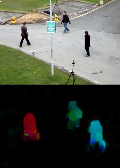
Figure 1 – Not the kind of optical flow we are talking about.
Source: https://docs.opencv.org/4.x/d4/dee/tutorial_optical_flow.html

What kind of optical flow are we talking about then? Name it as you like, since it does not have a broadly used name: feature tracking, sparse (please, no) optical flow, corner optical flow, etc. The key idea is: we are tracking specific points (corners) across a video. For this case, there is a widely used, robust, OpenCV-native algorithm called Lucas-Kanade method. That’s what we’ve used in the video in the beginning of the post.

The first thing you need to do when you ask the Lucas-Kanade method to track a corner is… to identify the corner in the image. Fortunately, OpenCV has an implementation of the Shi-Tomasi corner detection algorithm, which finds potentially good points in the initial frame of a video and provides them in a format ready to be passed to the Lucas-Kanade method. Voilà: that’s what the script in the video does.

The code is available below and was slightly adapted from this OpenCV doc page. If you’re eager to reproduce exactly what you see in the video, here’s a link to the input video at Google Drive.

import numpy as np
import cv2 as cv
import matplotlib.pyplot as plt

cap = cv.VideoCapture('videok.mp4')
# params for ShiTomasi corner detection
feature_params = dict( maxCorners = 5,
                       qualityLevel = 0.3,
                       minDistance = 7,
                       blockSize = 7 )
# Parameters for lucas kanade optical flow
lk_params = dict( winSize  = (15, 15),
                  maxLevel = 2,
                  criteria = (cv.TERM_CRITERIA_EPS | cv.TERM_CRITERIA_COUNT, 10, 0.03))
# Create some random colors
color = np.random.randint(0, 255, (100, 3))
# Take first frame and find corners in it
ret, old_frame = cap.read()
old_gray = cv.cvtColor(old_frame, cv.COLOR_BGR2GRAY)
p0 = cv.goodFeaturesToTrack(old_gray, mask = None, **feature_params)
# Create a mask image for drawing purposes
mask = np.zeros_like(old_frame)
list_x = list()
list_y = list()
while(1):
    ret, frame = cap.read()
    if not ret:
        print('No frames grabbed!')
        break
    frame_gray = cv.cvtColor(frame, cv.COLOR_BGR2GRAY)
    # calculate optical flow
    p1, st, err = cv.calcOpticalFlowPyrLK(old_gray, frame_gray, p0, None, **lk_params)
    # Select good points
    if p1 is not None:
        good_new = p1[st==1]
        good_old = p0[st==1]
    # draw the tracks
    for i, (new, old) in enumerate(zip(good_new, good_old)):
        a, b = new.ravel()
        c, d = old.ravel()
        mask = cv.line(mask, (int(a), int(b)), (int(c), int(d)), color[i].tolist(), 2)
        frame = cv.circle(frame, (int(a), int(b)), 5, color[i].tolist(), -1)
    list_x.append(a)
    list_y.append(b)
    img = cv.add(frame, mask)
    cv.imshow('frame', img)
    k = cv.waitKey(30) & 0xff
    if k == 27:
        break
    # Now update the previous frame and previous points
    old_gray = frame_gray.copy()
    p0 = good_new.reshape(-1, 1, 2)
cv.destroyAllWindows()

plt.plot(list_x, list_y)
plt.axis('equal')
plt.title('Estimated trajectory')
plt.xlabel('x [pixels]')
plt.ylabel('y [pixels]')